Lemniscate of Bernoulli
In geometry, the lemniscate of Bernoulli is a plane curve defined from two given points F1 and F2, known as foci, at distance 2a from each other as the locus of points P so that PF1·PF2 = a2. The curve has a shape similar to the numeral 8 and to the ∞ symbol. Its name is from lemniscus, which is Latin for "pendant ribbon". It is a special case of the Cassini oval and is a rational algebraic curve of degree 4.
The lemniscate was first described in 1694 by Jakob Bernoulli as a modification of an ellipse, which is the locus of points for which the sum of the distances to each of two fixed focal points is a constant. A Cassini oval, by contrast, is the locus of points for which the product of these distances is constant. In the case where the curve passes through the point midway between the foci, the oval is a lemniscate of Bernoulli.
This curve can be obtained as the inverse transform of a hyperbola, with the inversion circle centered at the center of the hyperbola (bisector of its two foci). It may also be drawn by a mechanical linkage in the form of Watt's linkage, with the lengths of the three bars of the linkage and the distance between its endpoints chosen to form a crossed square.[1]
Contents |
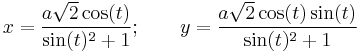
Equations
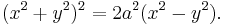
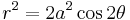 .
.
In two-center bipolar coordinates:

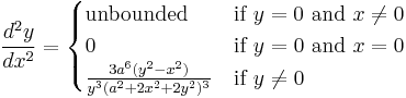
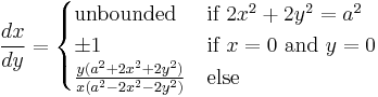
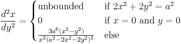
Derivatives
Each first derivative below was calculated using implicit differentiation.
With y as a function of x
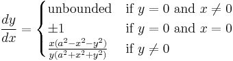
With x as a function of y
Curvature
Once the first two derivatives are known, curvature is easily calculated:
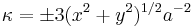
the sign being chosen according to the direction of motion along the curve. The lemniscate has the property that the magnitude of the curvature at any point is proportional to that point's distance from the origin.
Arc length and elliptic functions
The determination of the arc length of arcs of the lemniscate leads to elliptic integrals, as was discovered in the eighteenth century. Around 1800, the elliptic functions inverting those integrals were studied by C. F. Gauss (largely unpublished at the time, but allusions in the notes to his Disquisitiones Arithmeticae). The period lattices are of a very special form, being proportional to the Gaussian integers. For this reason the case of elliptic functions with complex multiplication by the square root of minus one is called the lemniscatic case in some sources.
See also
Notes
- ^ Bryant, John; Sangwin, Christopher J. (2008), How round is your circle? Where Engineering and Mathematics Meet, Princeton University Press, pp. 58–59, ISBN 9780691131184, http://books.google.com/books?id=iIN_2WjBH1cC&pg=PA58.
References
- J. Dennis Lawrence (1972). A catalog of special plane curves. Dover Publications. pp. 4–5,121–123,145,151,184. ISBN 0-486-60288-5.